
In September 1998, Long-Term Capital Management lost $4.6 billion in a few weeks. The spread models had been trained on normal-times correlations. The Russian default and the subsequent flight-to-quality made correlations historically around 0.3 converge to 1 within days. In When Genius Failed, Lowenstein cites the fund’s internal calculation of the probability of what happened:
“An event so freakish as to be unlikely to occur even once over the entire life of the universe […]”
The models were technically correct. They were just extrapolating confidence into a region of the space they had never seen. They had no “I don’t know” button.
My quant agent had the same problem, at incomparably smaller scale but with the same nature. I solved it this week.
In one sentence
Conservative degradation is the principle that says a model must have the right to abstain. When data is outside what it has seen, returning “I don’t know” is more useful than returning a spurious classification with mathematically high confidence.
The blind spot left after the data leakage fix
The previous post closed the chapter on Sharpe -1.14. The posterior became causal, the data leakage went away, the number became honest. But there was a blind spot the Sharpe didn’t show.
The 3-state Gaussian HMM always classifies. It receives a candle, computes the posterior over BULL/SIDEWAYS/BEAR, and returns the one with highest probability. By construction. If the features are in the normal training zone, fine. If they’re completely outside, it keeps classifying, and the posterior keeps summing to 1.
Concrete scenario: daily ATR 4x above the 90-day average, funding rate in historical extreme negative, volume 10x above normal. A spike the model simply has no reference point for. The HMM returns something like “BULL with 73% confidence”, because one of the three classes has to win.
Mathematically legitimate. Operationally dangerous.
What the literature calls this
I looked at the literature before implementing anything. Three threads converge.
Out-of-Distribution detection (computer vision, classical ML). The lineage starts with Hendrycks & Gimpel 2017 (“A Baseline for Detecting Misclassified and Out-of-Distribution Examples in Neural Networks”), showing that maximum softmax probability is already a reasonable confidence signal. Liang et al 2018 (ODIN) adds temperature scaling and adversarial perturbation, reducing false positive rate from 34.7% to 4.3%. Lee et al 2018 proposes Mahalanobis distance in feature space to capture covariance between dimensions. The three are the OOD canon.
Selective classification (statistics, pattern recognition). Chow 1957 already formalized the reject option in IRE Trans. Electronic Computers. In 1970 he derived the optimal error-reject curve. In 2017, Geifman and El-Yaniv brought the concept to deep learning with formal risk guarantee:
“We can achieve a target coverage with a guaranteed level of risk.”
The canonical metric for evaluating abstention is AURC (Area Under Risk-Coverage curve): shows how error falls as the model is allowed to reject more cases.
Critical systems with conservative degradation. Aviation has explicit regulation (FAA AC 25.1329-1B): autopilot must alert when envelope protection is invoked and disengage in off-nominal conditions. SAE J3016 (autonomous driving) defines Operational Design Domain (ODD) and requires the system to exit operation or request takeover when operating outside it. The principle is the same: a model trained for conditions X does not operate in Y, it alerts and returns control.
Trading benefits from this vocabulary. It was what was missing.
Someone has done this in finance
Two precedents to anchor on.
Kritzman and Li 2010 (“Skulls, Financial Turbulence, and Risk Management”, Financial Analysts Journal). They define the Turbulence Index as the multivariate Mahalanobis distance of returns against historical mean and covariance. Central quote:
“The more asset returns, volatilities and correlations differ from their historical norms, the more likely it is that these differences result from a significant market event rather than from random noise.”
Empirically the index aligns with 1987, the 1998 Russian default, 9/11, and the 2008 crisis. Turbulence is persistent, which justifies abstaining by windows, not by isolated tick.
Chalkidis et al 2021 (“Trading via Selective Classification”, ACM ICAIF, arXiv 2110.14914). This paper is the direct case of what I did. A binary up/down classifier becomes a strategy that only takes a position when it’s confident, and abstains when it’s not. Empirical result: smaller coverage with same risk improves Sharpe. The abstract’s quote:
“Selective classifiers give rise to trading strategies that do not take a trading position when the classifier abstains.”
Selective classification in trading is not my insight. It’s a documented topic at ACM. What was missing was bringing it to my HMM.
How I implemented it
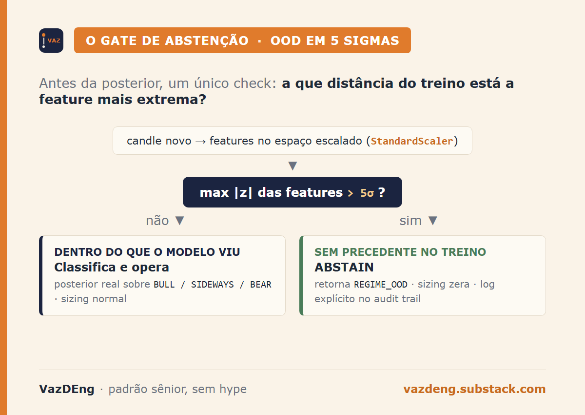
The HMM features pass through StandardScaler before training. In the scaled space, each feature’s mean is zero and standard deviation is one. Any new candle with one feature at very high absolute z-score is, by definition, outside the distribution the model has seen.
Threshold at 5 sigmas (conservative, crypto has fat tails). Static method on MarketRegimeHMM:
@staticmethod
def is_ood(x_scaled_row, threshold=OOD_SIGMA_THRESHOLD):
    if x_scaled_row.size == 0:
        return False
    return bool(np.nanmax(np.abs(x_scaled_row)) > threshold)
And predict_state checks before calling the posterior:
if self.is_ood(last_features):
    logger.warning("OOD detected: max |z| = %.2f > %.1f. Abstaining.",
                   max_dev, OOD_SIGMA_THRESHOLD)
    return REGIME_OOD, 0.0, {REGIME_OOD: 1.0}
The downstream decision (decide_position in layer 4) already had a lookup in REGIME_MULTIPLIER. I added "OOD": 0.0 as defense in depth, plus an explicit “ABSTAIN” log to make it visible whenever the system chose not to operate.
70 tests passed, plus 2 new ones covering the OOD path. Full suite in 6 seconds.
| Scenario | Before | After |
|---|---|---|
| Features inside distribution | Classifies BULL/SIDEWAYS/BEAR with real posterior | Same |
| Features 5+ sigmas outside (rare) | Classifies anyway, with spurious posterior | Returns OOD, sizing zeros |
| Log of the OOD tick | No distinction | “ABSTAIN: regime without playbook (OOD, conf=0.000)” |
| Trade opened in anomalous condition | Possible, with 2% cap | Impossible |
Why 5 sigmas, not 3
Threshold choice is where theory meets real crypto data. In perfectly Gaussian features, 3 sigmas would cover 99.73% and be reasonable. Crypto is not Gaussian. Realized volatility, funding rate, and DI spread have heavy tails. Bulla 2011 (Quantitative Finance) already showed that Gaussian HMM underestimates tails in financial returns, proposing Student-t instead.
At 5 sigmas, the detector fires only when the tick is in genuinely unprecedented region. At 3, it would fire on big but historical moves, generating excessive abstention. The next iteration is to swap univariate z-score for multivariate Mahalanobis (captures correlation between features), which is exactly what Kritzman-Li did in 2010 for returns.
What changed in my sleep
The most useful number for me isn’t the increase or decrease in Sharpe (I’ll measure in backtest next week). It’s this:
Before, when the agent took a position overnight and I woke up with Telegram blinking, I needed to open the auditor and read decision by decision to understand if the model had any logic at that moment or if it was guessing in chaotic market.
Now, if the system abstains, the log says ABSTAIN. If it operates, it’s because it was in territory it has seen. The question “does this decision have a basis?” became binary: there’s an ABSTAIN log before it, or there isn’t.
Nick Leeson, Jérôme Kerviel, LTCM, Knight Capital. The history of operational losses in finance almost always has the same pattern: a system continuing to make decisions when it shouldn’t. The cost of “I don’t know” has always been cheaper than the cost of “I thought it was”.
Anti-patterns to avoid
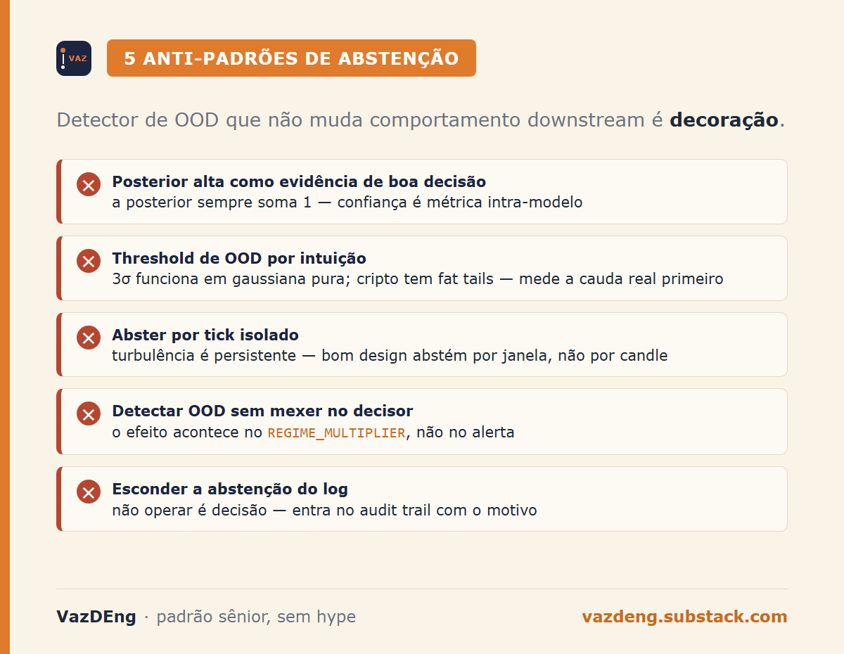
- Accepting high posterior as evidence of good decision. An HMM’s posterior always sums to 1. Confidence is intra-model metric, not evidence that the model understands what it’s seeing.
- Using OOD threshold based on intuition, not on distribution. 3 sigmas works in pure Gaussian. Crypto is not Gaussian. Measure the real tail of your data first.
- Abstaining on isolated tick and going back to operating on the next. Turbulence is persistent. Good design abstains by window, not by candle.
- Adding OOD without touching the decider. A detector that doesn’t change downstream behavior is decoration.
REGIME_MULTIPLIERis where the effect happens. - Hiding the abstention from the log. If the system preferred not to operate, that’s a decision. It must appear in the audit trail with reason, not silently.
The next chapter
The current version uses a single criterion (absolute z-score per feature). Two extensions are already in the backlog: Mahalanobis distance in the full space (captures covariance, which is what Kritzman-Li implemented for returns in 2010) and tick likelihood under the trained HMM (more sensitive, more expensive).
For now, what’s in production is the simple version. And it has already changed what I look at when I wake up.
Have you ever had a model return high confidence on a decision that shouldn’t have been made? Tell me on LinkedIn or subscribe to the newsletter to receive the next posts.